I have been following the discourse around RL, hearing a lot of terminology (like async RL, sample efficiency etc) and how people are using it to post-train models, and I did RL on smaller models like Qwen by following the docs of trl, unsloth. I could see the rewards going up, sometimes wiggling, sometimes 0, at times answer still being wrong at the end of training. I knew the math, the code, but I wanted to go deeper and had a lot of questions, like: what exactly changes in a model’s behaviour after RL? does it depend on how the pretraining was done? how stale can the rollouts be? - and many more. So I did some experiments and now writing this post to present those.
(The math and mechanics of algorithms like REINFORCE, PPO, GRPO etc. are all in an earlier post.)
To answer these questions what I really needed was an instrument: something I could train, poke at, and measure exactly, before and after RL (and preferably without spending money and all my free credits).
Why a real LLM makes a bad instrument (for my experiments)
Even with a smaller model, the overhead of running my experiments on real text data meant that I had to spend a lot of time waiting for results (or end up burning my free credits if I wanted them quickly).
But cost is only half of the problem - the bigger issue is what you cannot measure on a real model:
You only ever see sampled pass@k, and sampling is noisy. pass@k is the chance that at least one of k sampled tries is correct. On a real model you estimate it by actually sampling k completions per problem, so every number you get carries sampling noise on top of it. And the question I care about lives exactly where that noise is worst - at large k, where telling “the ceiling moved” apart from “we got lucky in sampling” needs an enormous number of samples.
You cannot read off exact probabilities. What I really want to know, per problem, is: what exact probability does the model assign to the correct answer, before and after RL? Getting that means teacher-forcing the correct answer and multiplying the per-token probabilities. That is feasible for a handful of problems on a big model, but not exhaustively over every problem in an eval set.
Statistically significant claims need repeats. RL runs wobble between seeds even with an identical config. One run of anything tells almost nothing - to claim an effect we need enough seeds to know our noise floor and check if the effect clears it (the intro post’s seeds and noise-floor section covers this). Thirty seeds of an RL run on a real model was not (and still isn’t) a good idea on my free credits.
So I built a tiny instrument(I might call it testbed too) which is fast to train, easy to play with, but running on the exact same underlying concepts, where I can run enough experiments to make claims with statistical significance instead of mistaking random occurrences for real effects.
The tiny instrument
The whole world of this instrument is arithmetic strings like 45+38=83 - and the model living in that world is small enough that anything I want to know about it can be measured exactly, not estimated.
The model. A completely standard decoder-only transformer (GPT-style), just tiny - pre-LayerNorm blocks, causal self-attention, GELU MLPs, learned positional embeddings. Nothing exotic, I did not want any finding to turn out to be an artifact of a weird architecture. The one deliberate omission is the KV cache - at sequence length ≤ 64 and ~10M parameters, recomputing the whole prefix at every generation step costs close to nothing.
| model spec | value |
|---|---|
| layers | 8 |
| heads | 8 |
| d_model / d_ff | 320 / 1280 |
| max sequence length | 64 |
| parameters | ~10M |
The vocabulary. Character-level, 20 tokens in total: the 17 task characters 0123456789+-*/=; (digits, the four operators, =, a ; scratchpad separator, and space), plus <pad>, <bos> and <eos>. There is no tokenizer, no BPE - every digit is its own token. This is not just for simplicity, it is what makes the key measurement of this post trivial: the probability the model assigns to an answer is a clean product of per-digit probabilities, so I can teacher-force the correct answer and read off the exact p(correct).
To be explicit about what this model does when treated as a policy network, at every step of generation it puts a distribution over these 20 tokens and picks one. In practice, answering a prompt like 387+456= means emitting a few digit tokens and then <eos> - and <eos> is itself a predicted action, the model decides where its answer ends. A model pretrained on direct answers has simply learned that digits-then-<eos> is the only thing to do after =.
The data. There is no dataset - problems are sampled on the fly. Draw operands with exact digit widths, format them as 45+38=, and the completion to learn is the answer 83; pretraining is plain next-character prediction on these strings (~1.28M examples over 5,000 steps). Every answer is an exact integer by construction - division samples the divisor and the quotient first, then sets a = b*q - so the verifier needs no math at all: extract the last run of digits from the generation and compare it to the true answer.
The pretraining mixture has 7 tasks - six everyday ones at equal weight, plus the RL target, 3-digit + 3-digit addition, whose weight is the one knob I deliberately turned down to ~1% of the mix. I intentionally created this gap so that the model sees the target just often enough to sometimes get it right, never often enough to become reliable at it.
| task | example | share of the mix |
|---|---|---|
| addition, 1+1 digit | 4+3=7 | ~16.5% |
| addition, 2+2 digit | 45+38=83 | ~16.5% |
| addition, 3+1 digit | 123+4=127 | ~16.5% |
| subtraction, 2−2 digit | 45-38=7 | ~16.5% |
| multiplication, 2×1 digit | 45*3=135 | ~16.5% |
| division, 2÷1 digit | 84/4=21 | ~16.5% |
| addition, 3+3 digit (the RL target) | 387+456=843 | ~1% |
Calibrating the instrument. Before running any experiment, I checked what this recipe actually produces:
- The six everyday tasks all reach 98-100% greedy accuracy. They also act as a retention gauge - every RL run re-checks them, so any collateral damage from training the target shows up immediately.
- The target sits at 26% greedy but 85% pass@64 - the model commits to the right answer only about 1 in 4 times, yet that answer is reachable 85% of the time if allowed 64 tries. So the base model gives correct answers, but not reliably, which is the gap that RL might close.
- To get the noise floor, I ran the same GRPO config 30 times, changing only the random seed, gives a spread of σ = 0.034 in final accuracy - about 5% of the mean. Every claim in this post is sized against that wobble.
And the first, most naive question I tried answering with this instrument was:
Does RL teach the model new things, or just make it better at what it already knew?
Sharpening or creating?
When RL improves a model on a benchmark, there are two possibilities:
- Creating - the model gained a capability it did not have before.
- Sharpening - the capability was already in the model’s distribution, and RL just concentrated probability mass on it.
The nice thing is that these two possibilities predict different pass@k curves(what happens to pass@k as k grows). Keep giving the model more tries, and at some point pass@k stops improving - every answer the model could realistically produce has already shown up. That plateau is the model’s capability ceiling. If RL only sharpens, one-try accuracy climbs toward the ceiling but the ceiling stays where it was. If RL creates, the ceiling itself rises - the tuned model reaches answers the base model could not, no matter how many tries the base gets.
The measurement. For each problem, I could teacher-force (src/exact_eval.py) the correct answer through the model and multiply the per-token probabilities.
To get the exact probability of the model producing that answer: p = P(answer + <eos> | prompt). Instead of letting the model generate freely, feed it the correct answer one character at a time and record the probability it assigns to each:
For 387+456= the true answer is 843, so p = P(8|387+456=) × P(4 | 387+456=8) × P(3 | 387+456=84) × P(<eos> | 387+456=843).
The model never gets to choose - the right character is forced into the context at every step, no matter what the model would have sampled. And once we have exact p, pass@k needs no sampling, we can write its closed form, since (1-p) is the probability of the model giving a wrong answer, the probability of getting at least one correct answer in k tries is:
$$\text{pass@k} = 1 - (1-p)^k$$Say a problem has p = 0.05. Then pass@8 = 1 − 0.95⁸ = 1 − 0.663 ≈ 34% - one try almost never works, but 8 tries succeed a third of the time. Compute this for every problem at every k and average, and you get the entire pass@k curve exactly - the thing that sampled pass@k merely estimates.
The experiment (scripts/05_x1_run.py):
- Freeze one pretrained substrate - every run below starts from these exact weights.
- Fix an eval set of 2000 target problems, sampled once with a fixed seed and reused everywhere.
- Teacher-force the base model on all 2000 problems → the before p-vector, measured once.
- Run GRPO on the target task: 500 updates, batch of 64 = 8 distinct problems × a group of 8 completions each, lr 1e-5. Repeat 30 times, changing only the random seed.
- After each run, teacher-force the tuned model on the same 2000 problems → 30 after p-vectors - plus a retention check on all six background tasks.
That gives one exact capability curve for the base and thirty for RL. The analysis (scripts/06_x1_analysis.py) sweeps k over powers of 2, from 1 to 1024. There is nothing special about 1024 - it is just far enough out that the curve has flattened: at k = 1024, even a problem the model gives only a 0.5% chance gets found with probability 1 − 0.995¹⁰²⁴ ≈ 99.4%, so the only answers still missing are ones the model essentially never produces.
This question is already being debated at scale - Yue et al. argue RLVR does not expand reasoning capacity beyond the base model, and Beren Millidge’s essay makes the information-theoretic case that RL moves very few bits and mostly brings out behaviours the base model already had. I came across these after doing the experiments(pushed June 14th) and when I was planning to write about it.
If RL is creating, the after-RL curve should end clearly above the base curve at k = 1024. If it is sharpening, the two curves should converge. Here are the observations:
Observation: the curves converge
The pass@1 accuracy more than tripled, but the ceiling(which is the pass@k at a k such that the model has exhausted everything that it can produce) barely moved 0.7 points.
500 GRPO updates, 30 seeds, and here are the exact pass@k numbers, before and after:
| metric | base | after RL |
|---|---|---|
| pass@1 | 18.4% | 65.4% |
| pass@64 | 84.8% | 94.3% |
| pass@1024 | 97.4% | 98.1% |
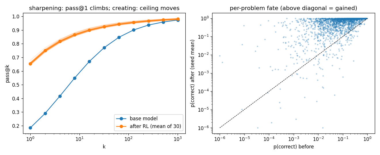
Left panel. The after-RL curve (orange) starts far above the base (blue) - one try now succeeds 65% of the time instead of 18% - but as k grows, the two curves meet. RL closed the gap between the floor and the ceiling; it did not raise the ceiling. The faint orange band around the mean is all 30 seeds - every run lands in the same place, so this is not one lucky training run. By the prediction we set up above: sharpening, not creating. Almost everything the tuned model does reliably, the base model could already do occasionally - RL redistributed probability mass toward answers that were already reachable.
Right panel. The same result, per problem: one dot per problem, its exact p(correct) before RL (x-axis) against after (y-axis, averaged over seeds), both on log scales. Almost every dot sits above the dashed diagonal, pushed up toward 1 - mass concentrating on the right answers, the sharpening happening problem by problem. But look at the dots hanging far below the diagonal: problems the base model solved, say, 1 time in 10 that the tuned model now solves essentially never. RL did not just lift problems - it destroyed some. Those dots are the thread the next two sections pull on.
Surprise 1: entropy collapse leaks to tasks RL never trained
RL only ever trained one cell: +(3,3). But the instrument has a full terrain map - think of a 4×6 grid: operations on one axis, operand widths on the other, every operation × digit-width combination (4 ops × 6 width pairs = 24 cells), each scored on greedy accuracy, exact p(correct), pass@64, and sampling entropy - how much the model explores when sampling at temperature 1. So after RL, I re-measured the entire map on the tuned models and diffed it against the base map (scripts/07_terrain_after_rl.py). One detail that matters: the after-measurement reuses the same random seeds, problem draws, and sample counts as the base measurement, so the numbers are comparable cell-for-cell - sampling noise cancels only when the problem sets match.
To be precise about what “entropy of a cell” means: at any context $s$ (the prompt plus whatever the model has generated so far), the model (or policy as I would interchangeably use) $\pi_\theta$ puts a distribution over the vocabulary $V$, whose Shannon entropy is
$$H\big(\pi_\theta(\cdot \mid s)\big) = -\sum_{v \in V} \pi_\theta(v \mid s)\,\log \pi_\theta(v \mid s)$$A cell’s entropy is that quantity averaged along the model’s own rollouts on that task $T$ - sample a problem, let the model generate, average the per-step entropies over the generated positions:
$$H(T) = \mathbb{E}_{x \sim T,\; y \sim \pi_\theta(\cdot \mid x)}\left[\frac{1}{|y|}\sum_{t=1}^{|y|} H\big(\pi_\theta(\cdot \mid x, y_{\lt t})\big)\right]$$(estimated with 256 rollouts per cell). Two things to note. It is on-policy - $y$ comes from the model itself, so this measures how spread out the model’s choices are along the paths it actually takes, which is exactly the “exploration” I care about. And it is in nats: uniform over the 10 digits would give $\ln 10 \approx 2.3$, a fully committed model gives 0 - so the numbers below, like 0.88 → 0.50, mean going from seriously weighing about three candidate digits at a typical step to mostly committing to one.
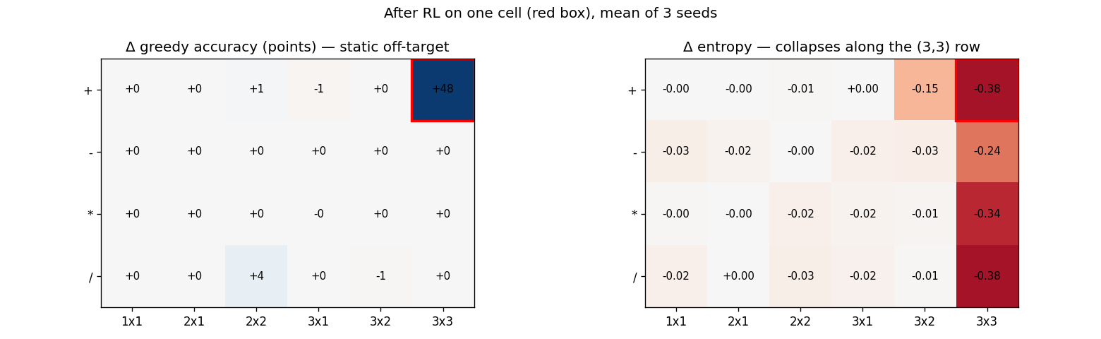
The left panel is expected: what the model can do changed only where RL trained. +48 points of greedy accuracy in the target cell (red box), ~0 everywhere else - the six background tasks retained fine.
The right one shows something I did not expect. The whole (3,3) column turns red. Take ÷(3,3) - a task RL never saw a single example of - its entropy dropped from 0.88 to 0.50(hence the -0.38), nearly half its exploration gone. Same for ×(3,3) and −(3,3), and it is consistent across seeds. Their accuracy did not move at all; only their willingness to explore did. Accuracy-based evals would never see this.
I didn’t expect this. RL never trained division, multiplication, or subtraction, but their entropy dropped anyway. The simplest explanation I have is shared surface structure: the target and the (3,3) column share operand and answer widths, so sharpening “commit to a 3-digit answer for a 3-digit problem” leaks across operations even though the arithmetic does not. And this matters beyond curiosity - recall from the intro post that RL can only reinforce what it samples. Entropy is what lets RL keep finding diverse rollouts. So sharpening one cell quietly drains the entropy from its structural neighbours, which predicts that a subsequent RL run on those neighbours starts from a worse exploration position.
Surprise 2: the same problems die in every run
Looking back at the dots below the diagonal in the figure 1, p(correct) is the exact probability of the model generating correct answer in one try. Using this probability, we can give status to problems:
- alive - p > 0.01, means 1 in 100 is correct per try. Such a problem is reachable in practice, at p = 0.01, 1024 tries find the answer with 1 − 0.99¹⁰²⁴ ≈ 99.99% chance.
- dead - p < 0.0001, means 1 in 10,000 is correct per try. Even 1024 tries usually miss it because 1 − 0.9999¹⁰²⁴ ≈ 10%. For any budget I would actually run, the model simply cannot do this problem.
So that means:
- If problem was alive before RL, and became dead after, that means it was killed.
- If a problem was dead before RL, and became alive after, that means it was revived.
Because of the 100x gap of alive and dead, a small wobble in p cannot fake a death or revival.
At the tails, the redistribution turns out to be two-sided and close to zero-sum:
| at the tails | fraction of problems |
|---|---|
| revived (p < 1e-4 → > 1e-2) | 0.27% |
| killed (p > 1e-2 → < 1e-4) | 0.24% |
| dead zone (p < 1e-4) | 0.65% → 0.82% |
Tiny fractions - each seed kills about 5 problems out of 2000. My first instinct was to dismiss this as noise. But 30 seeds let me ask a sharper question (scripts/08_x1_churn_structure.py): is each seed killing 5 random problems, or the same 5?
Two tests. First, cross-seed overlap. Take any two seeds and compare their killed-sets with the Jaccard index - size of the intersection over size of the union, so 1.0 means the exact same problems died and 0 means completely different ones. Now, 1750 of the 2000 problems were alive before RL and thus eligible to be killed; if each seed drew its ~5 victims at random from those 1750, two seeds would barely ever pick the same ones - expected Jaccard 0.0013. The observed value is 0.46 - about 355× the random baseline. Concentration makes it starker: across all 30 seeds, only 20 distinct problems were ever killed, 5 of them died in 10+ seeds, and one problem died in all 30 runs. Second, structure: compare the victims’ arithmetic features against the eligible pool they were drawn from -
| victims vs the eligible pool | victims | pool baseline | over-represented by |
|---|---|---|---|
| answer contains a 0 digit | 70% | 28% | 2.5× |
| units-digit carry | 85% | 42% | 2.0× |
| carries in all 3 columns | 35% | 15% | 2.3× |
Reading the first row: 70% of killed problems have a 0 somewhere in their answer, while only 28% of the eligible pool does - if death were random, those two numbers would match. (Each row is significant under a binomial test, p < 0.05.)
So the killing is not noise: RL reliably sacrifices the same hard minority - carry-heavy, zero-containing additions - to buy reliability on the majority. The revived problems, run through the same two tests, show nothing: no feature is significant, and their cross-seed overlap is only ~2.4× random (barely meaningful anyway, since just 13 problems were dead to begin with). I couldn’t find consistent structure in revivals, but kills were remarkably consistent.
Takeaways
We can now look at the pass@k curves and tell if the floor moved or the ceiling.
The same hard minority problems pay for the majority’s reliability in every run, and neighbouring tasks silently lose entropy that future RL could have used if we had to improve on those tasks. No accuracy-based eval can easily explain this.
These observations are not a quirk of our tiny setup, each finding has a counterpart measured on real LLMs, which is reassuring in both directions: the tiny setups tells us about the big models, and the big models validate the tiny setup, some references(claude/cursor helped me find these):
- Sharpening, not creating: Yue et al. found the same pass@k convergence on real reasoning benchmarks - RLVR models win at small k, base models catch up at large k.
- Entropy as the fuel: Cui et al. study entropy collapse in reasoning RL and even fit the trade explicitly - performance rises as entropy is exhausted, following $R = -a\,e^{H} + b$. Basically what we discussed as “draining fuel”, they wrote down as an equation.
- The killing: Wu et al.’s “The Invisible Leash” frames RLVR as support-constrained optimization and observes exactly the two-sided effect from Surprise 2 at scale - precision rises while empirical support shrinks, and the tuned model fails to recover correct answers the base model could reach.
- Zero-gradient groups: DAPO found all-correct/all-wrong groups wasteful enough at scale that one of its four core techniques, dynamic sampling, exists purely to filter them out.
Now an observation that also sets the stage for the post about my next experiments. By the last 20 updates of my runs, 53% of GRPO groups returned identical rewards - all 8 completions correct, or all 8 wrong - up from 43% at the start. Identical rewards mean zero advantage, zero advantage means zero gradient (the intro post covers why), so over half of compute that went into late-stage rollouts carried no learning signal at all. So if a group only teaches when the model finds at least one correct answer within 8 tries, then what the base model can reach in 8 tries is the real budget RL spends. So what exactly must pretraining supply for RL to work, and where does the extractable gain saturate? At scale, Shen et al. show post-RL performance is well-predicted from pretraining loss alone, my second experiment asks the same question where I can rerun pretraining itself - 18 base models, sweeping exactly one knob.
Code and full write-ups for all experiments: sky-2002/Tiny-RLVR.