After learning about RL for LLMs in research papers, some nice youtube playlists and reading some amazing blogs, I also wanted to write one, which can introduce RL for LLMs for someone who already knows LLMs, and one which I can refer anytime as a refresher. I have tried to build this blog right from softmax all the way to GRPO, and also tried to show calculations on a five-token toy example(which I will skip in one of the sections).
To set some base to build on, imagine that we have an LLM that solves a task sometimes, we want it to solve the task more often.
Language model is a probability distribution
During each step of autoregressive generation, an LLM produces a score (logit) for each token in the vocabulary, then converts those to probabilities with softmax. Consider the prompt 2+3= given to our toy model whose vocabulary is {0, 4, 5, 6, 15}. (Logits are deliberate multiples of $\ln 2$ so the softmax stays as fractions)
| Token | 0 | 4 | 5 | 6 | 15 |
|---|---|---|---|---|---|
| Logit ($z_i$) | ln2 | 3ln2 | 2ln2 | 2ln2 | ln2 |
| Token | 0 | 4 | 5 | 6 | 15 |
|---|---|---|---|---|---|
| (e^{z}) | 2 | 8 | 4 | 4 | 2 |
So the probabilities are:
| Token | 0 | 4 | 5 | 6 | 15 |
|---|---|---|---|---|---|
| Probability | 2/20 | 8/20 | 4/20 | 4/20 | 2/20 |
| 0.1 | 0.4 | 0.2 | 0.2 | 0.1 |
4 dominates at 0.4, the correct answer 5 sits at 0.2. But we want our model to have a higher probability for 5, to raise that 0.2.
Decoding rearranges, it does not relocate
Any decoding strategy draws from this same model (we will call it $\pi_\theta$ to indicate that it is parametrized by theta). A few that matter:
| Method | Effect on this $\pi_\theta$ | $P(5)$ |
|---|---|---|
| Greedy | always picks 4 | 0 |
| Sample, T=1 | draw from $\pi_\theta$ as-is | 0.20 |
| Temperature T=0.5 | sharpen → ∝ (4, 64, 16, 16, 4) → (1/26, 8/13, 2/13, 2/13, 1/26) | 2/13 ≈ 0.154 ↓ |
| Top-p, p=0.5 | keep {4,5} (5,6 tie at 0.2; assume the break goes to 5), renormalize to (0, 2/3, 1/3, 0, 0) | 1/3 ↑ |
Decoding alone moves accuracy from 0 to 1/3 without touching any weight. The trap is T=0.5: it lowers $P(5)$, sharpening goes toward the wrong mode, where the mass already was. Decoding rearranges. Training relocates.
SFT and RL exist to make correct answers more likely under the weights, not just under the sampler.
One answer, two strings (“5” vs “05”)
So far every completion is a single token. Real answers are sequences, and sequence probability is the product of its conditionals:
$$ \pi_\theta(y \mid x) = \prod_{t=1}^{T} \pi_\theta(y_{t} \mid x, y_{\lt t}) $$$$ \log \pi_\theta(y \mid x) = \sum_{t=1}^{T} \log \pi_\theta(y_{t} \mid x, y_{\lt t}) $$Extend the toy just enough to see this. Allow 1–2 digit answers plus EOS; the verifier does int(answer) == 5, so both "5" and "05" are correct. Step-1 distribution stays our $\pi_\theta$. After emitting 5, the model usually stops ($P(\mathrm{EOS}\mid 5)=0.8$). After emitting 0, it sometimes continues into 5 ($P(5\mid 0)=0.2$), then stops.
| Completion | Tokens | Probability |
|---|---|---|
"5" | 5, EOS | $0.2 \times 0.8 =$ 0.16 |
"05" | 0, 5, EOS | $0.1 \times 0.2 \times 1 =$ 0.02 |
Same semantic answer, 8× less probable, because every extra token multiplies by a factor $<1$, so log-probs add a penalty.
Making the right answer more likely
Decoding rearranges probability mass where it already sits. To relocate mass onto the correct answer, the weights have to move.
SFT
Supervised finetuning does the obvious thing: show the model (prompt, correct output) pairs and update with cross-entropy. Before that loss, let us see what entropy and cross-entropy are.
When some event happens very often, or is predictable, there is hardly any surprise(like we don’t see news of a sunrise, not much information gain), but when something happens rarely, it does have a surprise(we do see news of solar eclipse).
The surprise of an outcome $i$ under a distribution $p$ is given by ($-\log p_i$). The entropy of $p$ is the expected surprise:
$$ H(p) = \mathbb{E}_{i \sim p}[-\log p_i] = -\sum_{i} p_i \log p_i $$Cross-entropy is the same average, but the two roles split: for the things that actually happened, how startled was the model?
$$ L_{CE}(p, q) = \sum_{i=1}^{V} \underbrace{p_{i}}_{\text{did this happen?}} \cdot \underbrace{(-\log q_{i})}_{\text{model's surprise}} $$$p$ is the filter indicating which events count. $q$ is the scoring rule which tells how shocking that event is to the model. The multiply is not a mix of two distributions. Tokens which the label did not choose get $p_i=0$, so their surprise is not used. Training is not “be a good distribution everywhere”; it is don’t be surprised by the token that actually showed up.
Why is the model in $q$’s slot? Because ($-\log q_i$) is whose surprise is being measured so it has to be $\pi_\theta$. Order is $CE(p_{\mathrm{data}},\, \pi_\theta)$: the samples come from $p_{\mathrm{data}}$ and we calculate the expected value of the model’s surprise on those samples.
When $q = p$, CE collapses to $H(p)$. When $q \neq p$, it is always at least as large: $CE(p,q) = H(p) + D_{\mathrm{KL}}(p \| q)$, where
$$ D_{\mathrm{KL}}(p \| q) = \sum_i p_i \log \frac{p_i}{q_i} $$is the KL divergence - the extra surprise you pay for scoring $p$’s events with $q$ instead of $p$ itself (zero when $q = p$, positive otherwise, and not symmetric: swapping $p$ and $q$ changes it, which matters later for forward vs reverse KL).
The behavior to remember: wherever $p$ has mass but $q$ has almost none ($p_i > 0$ while $q_i \to 0$), the term $p_i \log(p_i/q_i)$ blows up, so KL stays large unless $q$ covers every place $p$ does. That extra term is forward KL, and it is the whole SFT objective once $p$ is a label.
In SFT, $q_i = \pi_\theta(i \mid x)$. For a given pair $(x,y)$ and token $y_t$ in $y$, $p$ is one-hot on $y_t$, so only one term survives: $1 \cdot (-\log \pi_\theta(y_t))$. Token 4 can have huge surprise but nobody cares, because 4 did not happen. CE is just the model’s surprise at the labeled token:
Same loss as negative log-likelihood of $y$ given $x$:
$$ \begin{aligned} NLL = -\log{\pi_\theta(y|x)} &= - \log{\prod_{t=1}^{T}\pi_\theta(y_{t}|x, y_{\lt t})} \\ &= - \sum_{t=1}^{T} \log{\pi_\theta(y_{t}|x, y_{\lt t})} \end{aligned} $$Both views say the same thing: make the tokens of the correct answer more likely, one token at a time.
One SFT step on the toy. Correct answer is 5, so:
The gradient w.r.t. the logits. Loss only cares about the correct token’s probability:
$$ L = -\log \pi_\theta(5) $$But $\pi_\theta$ comes from the logits $z$ via softmax:
$$ \pi_\theta(i) = \frac{e^{z_i}}{\sum_j e^{z_j}} \qquad\text{so}\qquad \pi_\theta(5) = \frac{e^{z_5}}{\sum_j e^{z_j}} $$Plug that in and simplify. The leading minus on the loss is the one that matters:
$$ L = -\log\left(\frac{e^{z_5}}{\sum_j e^{z_j}}\right) = -z_5 + \log\sum_j e^{z_j} $$Same thing as $L = -\log\pi_\theta(5)$, so $\partial L/\partial z_i = -\partial\log\pi_\theta(5)/\partial z_i$. Differentiate. Two cases:
- Correct logit ($i=5$): $\dfrac{\partial L}{\partial z_5} = -1 + \dfrac{e^{z_5}}{\sum_j e^{z_j}} = -1 + \pi_\theta(5) = \pi_\theta(5) - 1$
- Wrong logit ($i \neq 5$): $\dfrac{\partial L}{\partial z_i} = 0 + \dfrac{e^{z_i}}{\sum_j e^{z_j}} = \pi_\theta(i)$
(If the minus on $L$ were dropped, the correct-token entry would be $1-\pi_\theta(5)=+0.8$ which is the ascent direction on $\log\pi_\theta(5)$, i.e. REINFORCE with $r=1$. Descent on $L$ flips it.)
With $p$ = one-hot on 5, both cases are the same formula:
(“predicted minus true”). On the toy:
| Token | $\pi_\theta(i)$ | $p_i$ (one-hot) | gradient |
|---|---|---|---|
| 0 | 0.1 | 0 | +0.1 |
| 4 | 0.4 | 0 | +0.4 |
| 5 | 0.2 | 1 | −0.8 |
| 6 | 0.2 | 0 | +0.2 |
| 15 | 0.1 | 0 | +0.1 |
Gradient descent subtracts this, so the logit of 5 goes up and every other logit goes down. With learning rate 1, one step moves $\pi_\theta(5)$ from $0.2$ to $\approx 0.42$. Show the model the answer once, and the correct token roughly doubles its probability.
So SFT works, one step nearly doubled the right answer, and the same recipe scales, which is to show enough (problem, solution) pairs and the model learns the task, formats and all.
But, SFT is forward KL
Labels are not the scarce resource. Addition solutions are free(the point being - synthetic data is cheap). The problem is the loss.
Cross-entropy splits as
$$ CE(p, q) = H(p) + D_{\mathrm{KL}}(p \| q) $$$H(p)$ does not depend on the model. Minimizing CE is minimizing forward KL $D_{\mathrm{KL}}(p \| q)$, which is how much extra surprise you pay for using $q$ to score events that actually came from $p$.
Forward KL is brutal wherever $p$ has mass and $q$ does not, because ($-\log q_i$) blows up. So $q$ is forced to cover $p$. In SFT, $p$ is a spike on one labeled string (5, or "47+38=85"). A spike has $H(p)=0$, so
The model must put mass on that string. Every other token is treated as a mistake, including other answers that are also right. "05" verifies as 5, but under teacher forcing (at training time the model is fed the reference answer’s tokens as context and scored on predicting the next reference token, never its own output) the label is "5", so $p(\texttt{05})=0$ and SFT pushes its probability down while it shoves "5" up. This push-down is not a loss term on "05", the loss names only the label 5. It is the softmax coupling from the gradient section: raising $\pi(5)$ at step 1 necessarily drains mass from every other first token (that is the $\pi_i - p_i$ gradient), and since "05" must emit 0 first, draining $\pi(0)$ drains the whole "05" path. "05" simply loses the step-1 softmax competition to the label. (Concretely, for a two-token label like 85 on 47+38=: teacher forcing scores $P(8 \mid \texttt{47+38=})$, then feeds the true 8 and scores $P(5 \mid \texttt{47+38=8})$ ie always conditioning on the correct prefix, never on whatever the model itself would have guessed for the first digit.) That is not a data bug. That is what forward KL to a single reference is.
| SFT (forward KL) | RL (expected reward) | |
|---|---|---|
| Asks | match this labeled string | put mass on whatever scores |
| Other valid answers | penalized ($p=0$ there) | rewarded if the verifier says so |
| If the model never emits $y^*$ | still a gradient: raise $y^*$ anyway | no sample, no signal |
RL drops the reference $p$. Instead of covering a labeled string, raise $\pi_\theta$ on whatever the check scores. RLVR is just this setup with a verifier as the check.
def reward(prompt, completion):  # "47+38=", "85"
    return 1.0 if int(completion) == eval(prompt[:-1]) else 0.0
Checking is often cheaper than writing the answer, which is why math and code showed up first. Infinite synthetic labels would not change the objective: SFT would still be forward KL to those strings.
Sampling is acting: the RL view
Reframe the model in RL terms. When it is given 2+3= and samples 5, it did not just “decode a token”, it took an action. Out of five possible actions it committed to one, and the world (the verifier) responds with a score:
| RL term | In LLM land | In the toy |
|---|---|---|
| Policy $\pi_\theta$ | the model, as the distribution drawn from all along | $\pi_\theta = (0.1, 0.4, 0.2, 0.2, 0.1)$ |
| State | the prompt (plus tokens generated so far) | 2+3= |
| Action | sampling a token (or a whole completion) | picking 5 |
| Reward $r(y)$ | the verifier’s score for the finished answer | 1 if the answer is 5, else 0 |
| Rollout | one sampled completion together with its reward | sampled 4, got $r=0$ |
That is all RL is at this level: act → get scored → adjust. The rest of the field is vocabulary and variance reduction.
What are we optimizing?
SFT minimized a loss on given answers. RL maximizes the expected reward of the model’s own answers:
$$ J(\theta) = \mathbb{E}_{y \sim \pi_\theta(\cdot \mid x)}[r(y)] = \sum_{y} \pi_\theta(y \mid x)\, r(y) $$The toy is small enough to write this out in full:
$$ J(\theta) = 0.1 \cdot 0 + 0.4 \cdot 0 + 0.2 \cdot 1 + 0.2 \cdot 0 + 0.1 \cdot 0 = 0.2 $$Expected reward is just the probability of the correct answer which we have been trying to push up. SFT pushed it by pointing directly at the answer. RL has to push it knowing only the scores of whatever the model happens to sample.
Estimating $J$: Monte Carlo
The five-term sum above only works because the toy has five answers. A real model has $|\mathcal{V}|^L$ possible completions, for example, for Qwen, vocab $\sim 150\mathrm{k}$, even length-2 is already billions. The sum cannot be written down. So estimate it by sampling.
Draw $G$ independent completions from the model, score each with the verifier, average:
$$ \hat{J} = \frac{1}{G}\sum_{i=1}^{G} r(y_i), \qquad y_i \sim \pi_\theta(\cdot \mid x) $$That is Monte Carlo: replace an intractable expectation with an average over samples. On the toy, each $r(y)$ is a coin flip that lands $1$ with probability $J=0.2$. So $\hat{J}$ is just “fraction of the $G$ samples that got the answer right” which can be thought of as a random number whose law is $\mathrm{Binomial}(G, 0.2)/G$. One run of training sees one draw from that law. Across many independent groups the histogram of those draws is the four panels below: two spikes at $G=1$, still lumpy at $G=4$, and by $G=64$ the CLT bump $\mathcal{N}(J,\, J(1-J)/G)$ (orange) is a decent picture of it. The thing that has to get large for the bell is $G$ inside one average, not how many $\hat{J}$s you look at.
The width of that bump is the noise of one training estimate. One sample has variance $J(1-J) = 0.2 \times 0.8 = 0.16$, so standard deviation $0.4$. Averaging $G$ independent flips shrinks the standard error by $\sqrt{G}$:
$$ \mathrm{SE}(\hat{J}) = \frac{0.4}{\sqrt{G}} $$| $G$ | SE | Meaning |
|---|---|---|
| 1 | 0.40 | one rollout: estimate is either 0 or 1 |
| 4 | 0.20 | typical error about ±0.20 around the true 0.2 |
| 8 | 0.14 | |
| 64 | 0.05 | getting usable |
More samples → quieter estimate. GRPO later also draws a group of rollouts per prompt, but for a different reason than shrinking this error: the group’s mean reward becomes a baseline that stands in for a value function, and the spread within the group is what turns rewards into per-sample advantages (both covered soon). Precisely estimating the scalar $J$ is not the point there.
What can $\hat{J}$ actually look like at $G=4$? Only five possible values, i.e. $0, \tfrac{1}{4}, \tfrac{1}{2}, \tfrac{3}{4}, 1$, depending on how many of the four samples are correct. With $P(\text{correct})=0.2$:
| # correct out of 4 | $\hat{J}$ | Probability |
|---|---|---|
| 0 | 0 | $0.8^4 =$ 0.4096 |
| 1 | 0.25 | 0.4096 |
| 2 | 0.50 | 0.1536 |
| 3 | 0.75 | 0.0256 |
| 4 | 1.00 | 0.0016 |
Two things jump out.
- The estimator is usually $0$ or $0.25$, rarely near the true $0.2$ in a single group of 4. Unbiased on average across many groups; noisy in any one group.
- About 41% of the time, all four samples are wrong. Then $\hat{J}=0$, and every reward in the group is $0$. No correct example in the batch, nothing to reinforce. That number comes back when GRPO builds advantages inside a group (a group with zero reward variation carries zero learning signal).
So a training run is a noisy estimate of a number this toy computes exactly. RL, at this level, is: estimate expectations cheaply, then differentiate them safely.
This is why a single RL run proves nothing. A run here means one full training - fix a seed, train through all $N$ steps, read off the final accuracy. That final number is itself a random draw: the per-step sampling noise above compounds over the whole run, so two runs of the identical setup with different seeds finish at visibly different accuracies purely by luck. To claim an intervention actually helped, you run several seeds, measure the noise floor (how much that final number wobbles run-to-run with nothing changed), and believe only an effect that clears that floor - a change smaller than the noise is not a result. The spread shrinks by the same $1/\sqrt{n}$ law we just saw for $G$, now in the number of seeds: halving the uncertainty costs four times the runs.
Estimating $J$ is the easy half. The hard half: $J(\theta)$ is defined through sampling. You cannot backpropagate through a dice roll.
The score-function trick
$J$ is the expected reward from a few sections ago, on the toy, the five-term sum that equaled $0.2$. Written as a sum over answers:
$$ J = \sum_y \pi_\theta(y)\, r(y) $$Want $\nabla J$: how to nudge each token’s logit so $J$ goes up. If this were a smooth function of the logits, just differentiate under the sum. Training never writes the sum: it samples a $y$, sees a reward, and has to update from that. But the sampled token is a discrete pick, so no gradient flows through it because sampling is effectively an argmax over the logits plus random noise, and an argmax has zero gradient.
The way out is algebraic, by rewriting the gradient of the probability using a log:
$$ \nabla \pi_\theta(y) = \pi_\theta(y) \cdot \nabla \log \pi_\theta(y) $$(because $\nabla \log \pi_\theta = \nabla\pi_\theta / \pi_\theta$). Plug into $\nabla J$:
$$ \begin{align*} \nabla J &= \sum_y \bigl(\nabla \pi_\theta(y)\bigr)\, r(y) \\ &= \sum_y \pi_\theta(y)\, r(y)\, \nabla \log \pi_\theta(y) \\ &= \mathbb{E}_{y \sim \pi_\theta}\bigl[ r(y)\, \nabla \log \pi_\theta(y) \bigr] \end{align*} $$That is the score-function identity (log-derivative trick / REINFORCE). In words:
The gradient of expected reward = expected value of (reward × gradient of log-probability of whatever was sampled).
No differentiating through the sample. Sample $y$, look up $r(y)$, push $\log\pi_\theta(y)$ up if $r$ was big, down if $r$ was small. “Make good outcomes more probable in proportion to how good they were” is an exact identity, not a heuristic.
What $\nabla\log\pi_\theta$ actually is
Same softmax derivative as in SFT. Suppose the sample was 5. Then $\log\pi_\theta(5)$ is what gets differentiated, and the two cases are:
- logit of
5itself: $\dfrac{\partial \log\pi_\theta(5)}{\partial(\text{logit of }5)} = 1 - \pi_\theta(5) = 1-0.2 = +0.8$ - logit of any other token, say
4: $\dfrac{\partial \log\pi_\theta(5)}{\partial(\text{logit of }4)} = 0 - \pi_\theta(4) = -0.4$
In one row: $\dfrac{\partial \log\pi_\theta(y)}{\partial(\text{logit of }i)} = \mathbf{1}_{i=y} - \pi_\theta(i)$. For sampled 5:
| Token | $\mathbf{1}_{\text{this}=5} - \pi_\theta$ |
|---|---|
| 0 | $0-0.1$ = −0.1 |
| 4 | $0-0.4$ = −0.4 |
| 5 | $1-0.2$ = +0.8 |
| 6 | $0-0.2$ = −0.2 |
| 15 | $0-0.1$ = −0.1 |
One rewarded 5 says: raise the logit of 5, lower everything else, the same direction as SFT. The reward $r$ just scales this vector. If $r=0$ (wrong answer), the whole contribution is the zero vector.
Exact gradient on the toy
$J$ is still $0.2$. The score-function says $\nabla J = \mathbb{E}[r\,\nabla\log\pi_\theta]$. Five possible samples; only 5 has $r=1$, so four of the five terms vanish, and the survivor is $\pi_\theta(5)=0.2$ times the vector above, giving $\nabla J = (-0.02,\,-0.08,\,+0.16,\,-0.04,\,-0.02)$. The logit of 5 goes up by $0.16$, 4 down by $0.08$: not a new $J$, just $0.2$ times the SFT-style direction.
That same result is worth writing as a one-line identity, because GRPO’s advantage reuses it directly. Expand the expectation on the logit of token $i$:
$$ \begin{align*} \frac{\partial J}{\partial(\text{logit of }i)} &= \sum_y \pi_\theta(y)\, r(y)\, \bigl(\mathbf{1}_{y=i} - \pi_\theta(i)\bigr) \\ &= \pi_\theta(i)\, r(i) - \pi_\theta(i)\sum_y \pi_\theta(y)\, r(y) \\ &= \pi_\theta(i)\, r(i) - \pi_\theta(i)\, J \\ &= \pi_\theta(i)\,(r(i) - J) \end{align*} $$First term: only the $y=i$ summand survives the indicator. Second term: $\sum \pi_\theta r$ is $J$ again, the same $0.2$ already sitting around. Check token 5: $0.2\cdot(1-0.2)=0.16$. Token 4: $0.4\cdot(0-0.2)=-0.08$. Same vector.
| Token | $\pi_\theta$ | $r$ | $r-J$ | how this logit moves |
|---|---|---|---|---|
| 0 | 0.1 | 0 | −0.2 | −0.02 |
| 4 | 0.4 | 0 | −0.2 | −0.08 |
| 5 | 0.2 | 1 | +0.8 | +0.16 |
| 6 | 0.2 | 0 | −0.2 | −0.04 |
| 15 | 0.1 | 0 | −0.2 | −0.02 |
Sanity check: the five entries sum to $0$. Softmax ignores a constant added to every logit ($e^{z+c}$ cancels), so $J$ does not change if every logit moves together. The five nudges have to add to $0$.
Gradient ascent on $J$ (maximize reward) with learning rate 1: add that vector to the five logits, then softmax. $\pi_\theta(5)$ goes $0.2 \rightarrow \approx 0.2366$. Same learning rate as the SFT step that went $0.2 \rightarrow 0.42$. RL’s step is much smaller because the signal is weaker because it is an average over what the model samples, not a direct shove on the labeled answer.
(With lr $=5$, RL also reaches $\approx 0.42$. Same destination is possible; the per-step signal is just scaled down.)
REINFORCE is weighted SFT on the model’s own samples
Look at the update direction again. SFT on label 5 does gradient descent on $-\log\pi_\theta(5)$, which is ascent on $\log\pi_\theta(5)$, direction $\mathbf{1}_5 - \pi_\theta$. REINFORCE, when it happens to sample 5 with $r=1$, uses exactly that direction, scaled by $r$.
So REINFORCE = SFT on samples the model itself produced, weighted by their rewards. Two deep differences from ordinary SFT:
- Who generates the data - the model, not a labeler. If the model never samples the right answer, there is nothing to reinforce (the 41% all-wrong groups from earlier).
- What weights it - the verifier score $r(y)$, not a one-hot that assumes this string is the answer.
That is why RL can use a checker instead of a written solution and why it is helpless when the correct answer has probability near zero.
The identity is clean. The estimator of that identity, from a handful of samples, is not. Wrong answers currently contribute nothing ($r=0$ → zero gradient), and even correct ones give noisy updates.
Baselines: wrong answers have to count
A sampled 4 has $r=0$, so REINFORCE multiplies $\nabla\log\pi_\theta$ by zero. The update is the zero vector. The model just said the wrong answer and learned nothing about it.
The fix is to subtract a baseline $b$ before multiplying:
$$ \nabla J = \mathbb{E}\bigl[(r(y)-b)\,\nabla\log\pi_\theta(y)\bigr] $$Pick $b=J=0.2$ which is the model’s own average reward. Then a wrong 4 has weight $0-0.2=-0.2$, not $0$. The update for that sample is
The logit of 4 goes down. The mistake is now a training signal: “that was worse than my average, do less of it.” A correct 5 still gets a positive weight, now $1-0.2=0.8$ instead of $1$, same direction, but slightly quieter.
That difference $r-b$ is the advantage: better than your own average, not “right” in absolute terms. GRPO will use the mean of the group as $b$. Same idea, local.
Subtracting $b$ does not change the true gradient
$$ \mathbb{E}\bigl[b\,\nabla\log\pi_\theta\bigr] = b\sum_y \pi_\theta(y)\,\nabla\log\pi_\theta(y) = b\sum_y \nabla\pi_\theta(y) = b\,\nabla\!\Bigl(\sum_y \pi_\theta(y)\Bigr) = b\,\nabla 1 = 0 $$So $\mathbb{E}[(r-b)\nabla\log\pi_\theta]=\mathbb{E}[r\nabla\log\pi_\theta]$. The exact table above is unchanged. Only the spread of the per-sample estimates changes.
What actually drops, and what does not
What does subtracting the mean actually buy? Each sample’s update weight is its advantage $r-b$, so the update depends on how much better than average a sample was, not on the raw numbers the grader prints. That last part is the real payoff, and the way to see it is to change the grader.
Suppose it writes 10 for wrong and 11 for right instead of 0 and 1. The true gradient must not care because we just saw that subtracting a constant leaves $\nabla J$ untouched and with the mean baseline $b=J=10.2$ it doesn’t. The weights are
$$ r-b = (10-10.2,\; 10-10.2,\; 11-10.2,\; \ldots) = (-0.2,\; -0.2,\; +0.8,\; \ldots) $$exactly the $-0.2$ / $+0.8$ we had with the 0/1 grader. The offset vanished.
Now drop the baseline and watch it break. Each sample’s weight becomes its raw reward: every wrong answer yanks its $\nabla\log\pi_\theta$ by 10, every right one by 11. On average these near-equal pulls still cancel to the correct gradient but each individual pull is huge, so the estimate from a handful of samples swings wildly. On this toy that is 788× more estimator variance than subtracting the mean. That immunity to the grader’s scale is what the baseline is for.
On plain 0/1 rewards the variance win by itself is small, about 1.4× over the whole gradient because 0 and 1 already sit close together, so there is barely any offset to cancel. The baseline earns its keep the moment rewards stop being clean, centered 0/1, which in practice they do. (The variance-minimizing constant here works out to almost exactly the mean, so using the mean captures nearly all of the benefit.)
The whole update loop, so far
Everything up to now as one loop: sample a group, score it, turn scores into advantages, push each sample by its advantage.
for step in range(num_steps):
    ys      = [sample(pi_theta, x) for _ in range(G)]  # G answers to "2+3=", from the CURRENT policy
    rewards = [reward(x, y) for y in ys]               # verifier: 0/1
    adv     = [r - mean(rewards) for r in rewards]     # advantage; baseline = group mean
    g = mean(A * grad_logpi(y) for A, y in zip(adv, ys))  # grad_logpi(y) = onehot(y) − pi_theta
    theta = theta + lr * g                             # gradient ASCENT: maximize reward
Rollouts are expensive: this loop takes one gradient step per group, then throws the completions away.
On the toy at G=8, a step draws a couple of correct 5s among mostly 4s: the advantage tags the 5s positive and the 4s negative, and the update nudges the logits so $\pi_\theta(5)$ climbs and $\pi_\theta(4)$ falls. Run it and the 0.2 goes up.
That group-mean baseline is already GRPO’s “group-relative advantage.” What separates this from full GRPO is efficiency. Name the policy that generated a group $\pi_{\mathrm{old}}$ and the policy after an update $\pi_{\mathrm{new}}$: here ys is drawn fresh from the current policy every step and thrown away, so $\pi_{\mathrm{old}}$ and $\pi_{\mathrm{new}}$ stay in lockstep, the loop is always on-policy, and always paying full sampling cost. Reusing one group for several updates would break that lockstep ($\pi_{\mathrm{old}} \neq \pi_{\mathrm{new}}$), and making stale samples still count is exactly the next section.
Reusing rollouts: importance sampling
The completions were drawn from $\pi_{\mathrm{old}}$. After an update the model is $\pi_{\mathrm{new}}$. Those samples are not from the current policy but they still know something, if you reweight them.
The identity is just multiplying and dividing by the same number:
$$ \mathbb{E}_{y\sim\pi_{\mathrm{new}}}[f(y)] = \sum_y \pi_{\mathrm{new}}(y)\, f(y) = \sum_y \pi_{\mathrm{old}}(y) \cdot \frac{\pi_{\mathrm{new}}(y)}{\pi_{\mathrm{old}}(y)} \cdot f(y) = \mathbb{E}_{y\sim\pi_{\mathrm{old}}}\!\left[\frac{\pi_{\mathrm{new}}(y)}{\pi_{\mathrm{old}}(y)}\, f(y)\right] $$Sample from the stale policy, multiply by the ratio $\pi_{\mathrm{new}}/\pi_{\mathrm{old}}$, get an unbiased estimate under the new one. $f$ can be reward, or $(r-b)\nabla\log\pi_\theta$ - same trick.
When the policies are close, it just works
One exact gradient step on the toy, learning rate $0.1$:
| Token | $\pi_{\mathrm{old}}$ | $\pi_{\mathrm{new}}$ | ratio |
|---|---|---|---|
| 0 | 0.10 | 0.0999 | 0.999 |
| 4 | 0.40 | 0.3973 | 0.993 |
| 5 | 0.20 | 0.2035 | 1.017 |
| 6 | 0.20 | 0.1994 | 0.997 |
| 15 | 0.10 | 0.0999 | 0.999 |
Ratios sit in $[0.993, 1.017]$, very close to 1. The full sum $\sum \pi_{\mathrm{old}}\cdot\mathrm{ratio}\cdot r$ recovers $\pi_{\mathrm{new}}(5)=0.2035$ exactly but that exactness is not what closeness buys. That sum is an identity; it comes out right for any drift (the wild case below reproduces its $0.5$ just as exactly). What closeness buys is that a sampled estimate barely differs from on-policy: with every ratio ≈ 1, a handful of draws from $\pi_{\mathrm{old}}$ land almost exactly where draws from $\pi_{\mathrm{new}}$ would, so the reweighting adds almost no noise.
When they drift, the correction overcompensates
Want \(J\) under the new model. New model gets 5 right half the time, so the answer is \(0.5\). But the rollouts in hand were drawn from an old model that almost never says 5 (\(5\%\)).
The ratio tries to fix that: “when old does emit 5, new would have emitted it \(0.50/0.05=10\) times as often, so count this sample as ten.”
| Token | old | new | ratio = new/old |
|---|---|---|---|
| 0 | 0.60 | 0.20 | 0.33 |
| 4 | 0.15 | 0.10 | 0.67 |
| 5 | 0.05 | 0.50 | 10 |
| 6 | 0.10 | 0.10 | 1 |
| 15 | 0.10 | 0.10 | 1 |
The full sum is still exact: $\sum \pi_{\mathrm{old}}\cdot\mathrm{ratio}\cdot r = 0.05 \times 10 = 0.5$. The trouble is you never get to average over all of $\pi_{\mathrm{old}}$; you get \(G=8\) draws. Reward is 1 only on 5, so multiply each by its ratio:
- No
5in the eight (happens \(0.95^8 \approx 66\%\) of the time): every term is 0, so \(\hat{J}=0\). - One
5: that term is \(10 \times 1\), the other seven are 0, so \(\hat{J}=10/8=1.25\). - Two
5s: \(\hat{J}=20/8=2.5\).
The estimate is \(0\), or \(1.25\), or \(2.5\), … never \(0.5\). Average those over infinite groups and you do get \(0.5\). That is all “unbiased” means. One group is still a miss or an overshoot.
If those eight had been drawn from new, about four would be correct and \(\hat{J}\) would sit near \(0.5\). Same target, no \(\times 10\). The stale samples make the estimator 19× noisier.
So: IS is a correction factor. It is exact on average and wild on any one batch unless old and new still agree, like the \(0.1\) step above.
How near is near: the trust region
Importance sampling reuses a group only while $\pi_{\mathrm{new}}$ stays close to the $\pi_{\mathrm{old}}$ that produced it, the drift example showed the estimator going wild the moment they part. “Close” needs a number, and the natural one is the KL between them:
$$ D_{\mathrm{KL}}(\pi_{\mathrm{old}} \,\|\, \pi_{\mathrm{new}}) $$zero when the policies match, growing as they separate. TRPO takes this literally: at each step, maximize the importance-weighted reward subject to $D_{\mathrm{KL}}(\pi_{\mathrm{old}}\|\pi_{\mathrm{new}}) \le \delta$ which is a hard leash of radius $\delta$ around the old policy. Inside the leash the reused samples are trustworthy; the constraint simply forbids the runaway step.
It works, and the price is stiff. A KL-constrained step is a second-order problem: you need the curvature of the KL (the Fisher information matrix) and solve it with conjugate gradients plus a line search, every update. For a model with billions of parameters that is a great deal of machinery to avoid one bad step.
The cheaper leash: PPO’s clip
PPO keeps the goal (don’t let one reused batch drag the policy too far) and drops the constrained solve for something first-order and blunt. The reused-sample update already weights each advantage by the ratio $\rho = \pi_{\mathrm{new}}(y)/\pi_{\mathrm{old}}(y)$. PPO just clips that ratio into $[1-\epsilon,\,1+\epsilon]$ and maximizes
$$ J^{\mathrm{PPO}} = \mathbb{E}\Big[\min\big(\rho\,A,\ \ \mathrm{clip}(\rho,\,1-\epsilon,\,1+\epsilon)\,A\big)\Big] $$(the PPO paper writes this as $L^{\mathrm{CLIP}}$; same thing, an objective to push up).
One rule makes the whole thing make sense: the clip only brakes a step in the direction the update is trying to move the ratio, and never brakes the correction back toward 1. A good action ($A>0$) wants its ratio pushed up; a bad action ($A<0$) wants it pushed down. Overshoot the band in that wanted direction and the objective goes flat.
Good action first. Token 5 has advantage $A=+0.8$ (its $r-b$ from the baseline section), and reuse has pushed its ratio to $\rho=2.0$ which means the model now likes 5 twice as much as the policy that sampled it. With $\epsilon=0.2$:
- unclipped: $\rho A = 2.0 \times 0.8 = 1.6$
- clipped: $\mathrm{clip}(2.0,\,0.8,\,1.2)\,A = 1.2 \times 0.8 = 0.96$
- $\min(1.6,\ 0.96) = 0.96$
Past $\rho=1.2$ the objective is flat (gradient zero): no extra reward for pushing 5 more than 20% beyond where $\pi_{\mathrm{old}}$ had it. Promotion is deliberately subtle.
Bad action: where the flat side flips. Token 4 is wrong, $A=-0.2$; the update wants its ratio down.
- Reuse drives $\rho$ below the band, say $\rho=0.5$: $\min(0.5\cdot(-0.2),\ 0.8\cdot(-0.2)) = \min(-0.10,\,-0.16) = -0.16$ (the clipped term), flat. The objective flattens once $\rho$ drops past $0.8$ — the mistake already 20% less likely than under $\pi_{\mathrm{old}}$ — and $\rho=0.5$ is well past that, so the clip stops us punishing it further on stale evidence.
- But if the model still over-likes the mistake, $\rho=2.0$: $\min(2.0\cdot(-0.2),\ 1.2\cdot(-0.2)) = \min(-0.40,\,-0.24) = -0.40$ (the unclipped term), and it grows with $\rho$. A confidently-wrong action is pushed down hard, with no cap.
Same band, opposite behavior by sign:
| ρ below band | ρ above band | |
|---|---|---|
| good action (wants ↑) | full push up | flat (promotion capped) |
| bad action (wants ↓) | flat (can’t over-punish) | full push down (heavy) |
So the clip is subtle with optimism, heavy on confident mistakes: a good action can’t be chased more than $+\epsilon$, but a mistake the model still favors is suppressed in proportion to how much it favors it.
$\min$ is used because it makes the surrogate pessimistic so always the less-favorable of clipped and unclipped is picked, so an overshoot in the wanted direction is never rewarded, only ignored, while a correction back toward 1 keeps its full gradient.
So PPO is a soft, one-sided trust region enforced per update, no Fisher matrix in sight. The KL you would have constrained in TRPO becomes a diagnostic you watch, $D_{\mathrm{KL}}(\pi_{\mathrm{old}}\|\pi_{\mathrm{new}})$ creeping up as you take more inner steps on one group.
There is a bias–variance trade hiding in this. The raw importance-sampled update is unbiased(averaged over enough samples it points the right way) but its variance explodes as the policy drifts (the wild estimates from the drift example). The clip caps that variance, and pays for it with a little bias: the clipped, pessimistic surrogate is no longer the exact gradient. Accepting a small, deliberate bias to kill a lot of variance is the whole reason it works(and it is why LLM RL is so touchy about staleness). A heavily-pretrained policy sits in a very precise spot, so even a little bias from stale, off-policy samples can drag it somewhere worse; the clip is the leash that keeps that drift in check.
The critic, and why GRPO doesn’t use one
One piece of PPO is still open: the baseline. We subtracted the mean reward $b$ and called $r-b$ the advantage, but where does $b$ come from at scale, where you cannot enumerate outcomes?
The principled answer is a value function $V(s)$: the reward a state should expect. Subtract it and the advantage reads “did this beat what this state normally gets.” In the toy the “state” is just the prompt 2+3=, the reward is terminal (0/1 at the very end), so $V(\texttt{2+3=})$ is nothing more than that prompt’s success probability. Two ways to get it:
- Learn it. Train a second network $V_\phi$ next to the policy to predict it, this acts as the critic to the policy’s actor. This is PPO. In genuine multi-step RL the critic earns its keep, because reward can arrive midway through a trajectory and must be spread back over the steps that earned it. RLVR, with one verifier score per finished answer, barely needs it.
- Estimate it by sampling. For a fixed prompt, draw a group of completions and use their mean reward as $V$. No second network as we then pay in samples instead of parameters.
That second route is GRPO. “Group-relative” means the baseline is the group’s own mean, hence local, and the advantage is $r_i - \mathrm{mean}(\text{group})$, usually also divided by the group’s std which standardizes the scale so an easy prompt and a hard one contribute comparable gradients, instead of whichever happens to have the larger reward spread dominating the update. It drops the critic entirely.
Credit assignment: GAE (stepping off the toy)
Everything so far had a single step of sampling one answer and getting one reward which is exactly why the arithmetic toy stayed hand-checkable: with one step there is nothing to spread. Real trajectories aren’t like that, so this section leaves the five-token toy for a small made-up one, just to see the piece PPO’s critic is really built for.
The idea to hold onto is credit assignment. A soccer team wins 1–0: the striker scored, but the midfielder’s pass set it up and a defender won the ball three plays earlier, so to reward the team fairly you have to trace credit back through the whole sequence that produced the goal, not just hand it to whoever touched the ball last. Multi-step RL has exactly this problem: a reward that lands at the end has to be shared out among the earlier actions that made it possible. GAE is a recipe for doing that spreading.
Picture an episode of several steps: state $s_0$, an action, reward $r_0$; then $s_1$, an action, reward $r_1$; and so on. The return from step $t$ is the discounted sum of everything that follows,
$$ G_t = r_t + \gamma\, r_{t+1} + \gamma^2 r_{t+2} + \cdots $$with a discount $\gamma \in (0,1]$ that says how much a reward counts later versus right now. Think of it as patience. At $\gamma$ near 1 a reward ten steps away is worth almost as much as one this instant, so credit reaches far back to whatever set it up; at a small $\gamma$ the model is myopic, meaning that distant rewards are heavily shrunk, and credit for a reward barely reaches past the steps just before it. So $\gamma$ sets the horizon over which actions and rewards are linked.
The value $V(s_t)$ is the expected return from $s_t$, and the advantage of the action actually taken is $G_t - V(s_t)$ which tells us whether actual return beat the expected return, the same move as before, now once per step.
The hard part is credit: a reward at step 5 might be owed to the action at step 1. There are two ways to judge how good a single step was, and they pull against each other.
One extreme is the full return $G_t$: take the step, then watch everything that actually happens afterward and score the step by the real total. Honest, but it soaks up all the downstream luck, so it is noisy (high variance).
The other extreme leans on the critic. Recall $V(s)$ is the critic’s guess of how well things go from state $s$. Rather than wait for the whole future, judge the step by a cheaper question - did it leave things better than the critic expected? That one-step surprise is the TD error $\delta_t$ (temporal difference): the critic’s guess after the step minus its guess before, corrected by the one real reward you actually saw.
Concretely: before the step the critic expects $V(s_t)$; you take the action, collect reward $r_t$, land in $s_{t+1}$ where it now expects $V(s_{t+1})$. So
$$ \delta_t = \underbrace{r_t + \gamma\, V(s_{t+1})}_{\text{guess after: one real reward + critic's read of the rest}} \;-\; \underbrace{V(s_t)}_{\text{guess before the step}} $$Positive $\delta_t$ means the step beat expectations (do more of that action); negative means it fell short.
So: the full return is honest-but-noisy, the TD error is quiet-but-critic-dependent. GAE dials between the two, as an exponentially-weighted sum of those one-step surprises:
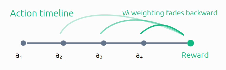
$$ \hat{A}^{\mathrm{GAE}}_t = \sum_{l=0}^{\infty} (\gamma\lambda)^l\, \delta_{t+l} $$The weight $(\gamma\lambda)^l$ fades each future surprise the further ahead it sits, and $\lambda \in [0,1]$ sets how fast:
- $\lambda = 0$: only $\delta_t$ survives — take the critic’s one-step read, ignore the rest. Quiet, critic-dependent.
- $\lambda = 1$: every surprise counts, telescoping into the actual return minus $V(s_t)$. Honest, noisy.
In soccer terms, $\lambda$ asks: credit the pass by the coach’s instant read (“dangerous position”), or wait to see whether the attack actually scores? Trust the coach and every identical pass gets the same verdict(low variance) but you inherit whatever the coach is systematically wrong about (bias). Wait for the goal and you are right on average, but the verdict swings with all the downstream luck (high variance, no bias). Bias is a consistent tilt; variance is random scatter; $\lambda$ picks the mix.
$\gamma$ is a different knob, easy to confuse since both fade distant steps. $\gamma$ asks how much do I value a goal scored later?, $\lambda$ changes only how you estimate it. (That one $\gamma$ shows up wherever a future is valued: the return, the $V(s_{t+1})$ in $\delta_t$, and the $(\gamma\lambda)^l$ weights.)
We will use a three-step episode as a made-up trajectory, not the arithmetic toy, since that one has only a single step. Take $\gamma = 1$, rewards $r = (0, 0, 1)$ (nothing until a win at the end), and a critic already predicting $V = (0.5, 0.6, 0.7)$ along the way. Each $\delta_t = r_t + V(s_{t+1}) - V(s_t)$ (terminal $V = 0$):
| step $t$ | $r_t$ | $V(s_t)$ | TD error $\delta_t$ | adv. $\lambda{=}0$ | adv. $\lambda{=}0.5$ | adv. $\lambda{=}1$ |
|---|---|---|---|---|---|---|
| 0 | 0 | 0.5 | 0.1 $\;(0{+}0.6{-}0.5)$ | 0.1 $\;(\delta_0)$ | 0.225 $\;(\delta_0{+}\tfrac12\delta_1{+}\tfrac14\delta_2)$ | 0.5 $\;(\delta_0{+}\delta_1{+}\delta_2)$ |
| 1 | 0 | 0.6 | 0.1 $\;(0{+}0.7{-}0.6)$ | 0.1 $\;(\delta_1)$ | 0.25 $\;(\delta_1{+}\tfrac12\delta_2)$ | 0.4 $\;(\delta_1{+}\delta_2)$ |
| 2 | 1 | 0.7 | 0.3 $\;(1{+}0{-}0.7)$ | 0.3 $\;(\delta_2)$ | 0.3 $\;(\delta_2)$ | 0.3 $\;(\delta_2)$ |
The advantage columns are just the TD errors added up with the $(\gamma\lambda)^l$ weights: $\lambda{=}0$ keeps only $\delta_t$, $\lambda{=}1$ sums every $\delta$ from $t$ onward, $\lambda{=}0.5$ fades each further one by half ($\tfrac12,\tfrac14,\dots$). (Here $\gamma{=}1$, so the weights are just $\lambda^l$.)
Read step 0 across its row: its credit climbs $0.1 \to 0.225 \to 0.5$ as $\lambda$ opens up. At $\lambda = 0$ the critic says step 0 barely helped; at $\lambda = 1$ it earns full credit for the eventual win (and the Monte-Carlo check agrees: $G_0 - V(s_0) = 1 - 0.5 = 0.5$). Step 2 stays $0.3$ whatever $\lambda$ is because there is no future beyond the last step to fold in, so the dial has nothing left to turn.
And then what do we do with it? Nothing new. Whatever $\lambda$ you pick, GAE hands back one number per step, the advantage $\hat{A}_t$ and that is the same advantage the policy-gradient update multiplies $\nabla\log\pi$ by, the one PPO’s clipped surrogate weights each token with. GAE only changes how that number is estimated; the update wrapped around it is exactly the one we already built. The whole detour was just to get a better $\hat{A}_t$ to plug back in.
All of that credit-spreading assumed we actually have per-step rewards to spread, and that is precisely the hard part. A verifier can only score a finished answer, it has no cheap, reliable way to say whether the token you emitted halfway through was “good.” We could train a separate model to grade partial work(a process reward model) but those are noisy, expensive, and tend to add bias that dilutes the very signal RL is after; a step that looks right can lead nowhere, and an odd-looking one can set up the win. So the robust, common choice is a single reward at the very end.
GAE does not flatten on its own. Even with one terminal reward and $\gamma = 1$, the $\lambda = 1$ column above came out $0.5, 0.4, 0.3$: different per step, because each subtracts its own $V(s_t)$. The flattening is a choice GRPO makes. With no intermediate rewards a per-token critic has almost nothing to learn, so rather than train one, GRPO replaces the whole per-state $V(s_t)$ with a single per-prompt baseline $b$, the group’s mean reward. Then every token’s advantage is $r - b$, identical down the sequence, and there is nothing left for $\lambda$ to interpolate.
GRPO, assembled
GRPO is REINFORCE with two swaps, the baseline becomes a group mean (no critic), and rollouts are reused under PPO’s clip:
for step in range(num_steps):
    # ── generate: freeze pi_old, sample a group ──
    pi_old  = freeze(pi_theta)
    ys      = [sample(pi_old, x) for _ in range(G)]        # G answers to "2+3="
    rewards = [reward(x, y) for y in ys]                   # verifier: 0/1
    A       = [(r - mean(rewards)) / (std(rewards) + 1e-8) # group-relative advantage
               for r in rewards]                           #   (mean = baseline, no critic)

    # ── learn: reuse the group for a few CLIPPED steps ──
    for _ in range(num_inner_steps):
        rhos = [pi_theta(y) / pi_old(y) for y in ys]       # rho = pi_new / pi_old, 1.0 on pass 1
        obj  = mean(min(rho * a, clip(rho, 1-eps, 1+eps) * a)
                    for rho, a in zip(rhos, A))            # PPO clipped surrogate
        theta = theta + lr * grad(obj)                     # ascent
That is the full GRPO update: group mean for the baseline, the clip for the trust region, a verifier for the reward (REINFORCE underneath it all), with the two swaps that make reuse safe and the critic unnecessary. Set num_inner_steps = 1 and every rho is 1, the clip never fires, and it reduces to the plain on-policy loop.
A couple of practical points the single-token toy hides. The ratio and clip are applied per token, not per whole sequence. And the length bias promised back at “5” vs “05” is real but it does not come from the clip; it comes from how the per-token losses are aggregated. GRPO averages each response’s loss over its own length, so a long wrong answer is penalized more gently, per token, than a short one, thus nudging the model toward ever-longer completions (the Dr. GRPO / DAPO critique), with the raw log-prob penalty from “05” adding to it. Separately, RLHF hangs a KL-to-reference term (the mode-seeking reverse KL) on top of the reward.
One training dynamic worth naming: entropy collapse. As RL sharpens the policy onto what already scores, $\pi$ can spike on a few tokens and stop exploring, and since RL only reinforces what it samples, a collapsed policy has nothing left to learn from. That is why practitioners watch entropy and sometimes add an entropy bonus to keep it spread.
Everything in one place
The whole arc is one idea that is to push probability toward what scores higher, refined step by step. Every RL variant below maximizes the same objective, expected reward $J(\theta) = \mathbb{E}_{y\sim\pi_\theta}[r(y)]$; they differ only in the per-batch surrogate they optimize and how safely they reuse samples. So each RL line below is written as a surrogate $J^{(\cdot)}$ you maximize over the sampled completions (held fixed $\hat{\mathbb{E}}$ is the average over that batch, so differentiating it gives the policy-gradient update); SFT is the one loss $L$ you minimize. The skeleton under each shows its loop, what it samples and whether a batch of rollouts buys one update or many.
SFT: imitate the labelled answer, token by token (minimize):
$$ L_{\mathrm{SFT}} = -\sum_t \log \pi_\theta(y_t \mid x, y_{\lt t}) $$for x, y in dataset: # external (prompt, answer) labels
theta -= lr * grad(-logpi(y, x)) # one step per batch, no sampling
REINFORCE: imitate the model’s own samples, weighted by reward (maximize):
$$ J^{\mathrm{REINFORCE}} = \hat{\mathbb{E}}_{y\sim\pi_\theta}\big[\, r(y)\,\log\pi_\theta(y) \,\big] \qquad\Rightarrow\qquad \nabla J = \hat{\mathbb{E}}_{y\sim\pi_\theta}\big[\, r(y)\,\nabla\log\pi_\theta(y) \,\big] $$for step in range(N):
ys = [sample(pi_theta, x) for _ in range(G)] # FRESH from the current policy
g = mean(r(y) * grad_logpi(y) for y in ys)
theta += lr * g # ONE update, then discard ys
REINFORCE + baseline: subtract a baseline $b$ so wrong answers also count; the weight becomes the advantage $A = r-b$ (maximize):
$$ J^{\mathrm{RF+baseline}} = \hat{\mathbb{E}}_{y\sim\pi_\theta}\big[\, (r(y)-b)\,\log\pi_\theta(y) \,\big] $$for step in range(N):
ys = [sample(pi_theta, x) for _ in range(G)] # still fresh, on-policy
b = mean(r(y) for y in ys) # baseline = group mean
g = mean((r(y) - b) * grad_logpi(y) for y in ys)
theta += lr * g # one update, then discard
TRPO: reuse rollouts from $\pi_{\mathrm{old}}$ (ratio $\rho = \pi_\theta/\pi_{\mathrm{old}}$), held on a hard KL leash (maximize, constrained):
$$ J^{\mathrm{TRPO}} = \hat{\mathbb{E}}_{y\sim\pi_{\mathrm{old}}}\big[\,\rho\, A\,\big]\quad\text{s.t.}\quad \hat{\mathbb{E}}_{y\sim\pi_{\mathrm{old}}}\big[D_{\mathrm{KL}}(\pi_{\mathrm{old}}\,\|\,\pi_\theta)\big]\le\delta $$for step in range(N):
pi_old = freeze(pi_theta)
ys = [sample(pi_old, x) for _ in range(G)]
# ONE constrained, second-order step:
# max mean(rho * A) s.t. KL(pi_old || pi_theta) <= delta
theta = trust_region_step(ys, A) # Fisher + conjugate gradient
PPO: drop the constrained solve; enforce the leash with a cheap clip (maximize):
$$ J^{\mathrm{PPO}} = \hat{\mathbb{E}}_{y\sim\pi_{\mathrm{old}}}\Big[\min\big(\rho\, A,\ \ \mathrm{clip}(\rho,\,1-\epsilon,\,1+\epsilon)\,A\big)\Big] $$for step in range(N):
pi_old = freeze(pi_theta)
ys = [sample(pi_old, x) for _ in range(G)]
for _ in range(K): # reuse the SAME batch K times
rho = pi_theta(y) / pi_old(y) # 1.0 on the first inner step
theta += lr * grad(mean(min(rho*A, clip(rho, 1-eps, 1+eps)*A)))
GRPO: PPO’s clip, but the advantage comes from a group of $G$ rollouts per prompt (no critic), applied per token (maximize):
$$ J^{\mathrm{GRPO}} = \hat{\mathbb{E}}_{y_i\sim\pi_{\mathrm{old}}}\Big[\tfrac{1}{G}\sum_{i=1}^{G}\min\big(\rho_i A_i,\ \ \mathrm{clip}(\rho_i,\,1-\epsilon,\,1+\epsilon)\,A_i\big)\Big] \;-\; \beta\, D_{\mathrm{KL}}(\pi_\theta \,\|\, \pi_{\mathrm{ref}}), \qquad A_i = \frac{r_i - \mathrm{mean}(\mathbf{r})}{\mathrm{std}(\mathbf{r})} $$for step in range(N):
pi_old = freeze(pi_theta)
ys = [sample(pi_old, x) for _ in range(G)] # G rollouts per prompt
A = [(r(y) - mean(r)) / (std(r) + 1e-8) for y in ys] # group-relative, no critic
for _ in range(K): # reuse the SAME group K times
rho = pi_theta(y) / pi_old(y)
theta += lr * grad(mean(min(rho*A, clip(rho, 1-eps, 1+eps)*A)))
# optional RLHF leash: - beta * grad(KL(pi_theta || pi_ref))
The trailing $-\beta\,D_{\mathrm{KL}}(\pi_\theta\|\pi_{\mathrm{ref}})$ is the optional RLHF reference leash: $\pi_{\mathrm{ref}}$ is the frozen pre-RL model (the SFT/base checkpoint, not the $\pi_{\mathrm{old}}$, which refreshes every step), and the term keeps $\pi_\theta$ from drifting too far from it (the mode-seeking reverse KL).
In one breath: SFT imitates a label; REINFORCE imitates model’s own reward-weighted samples; the baseline turns reward into advantage; TRPO/PPO make it safe to reuse those samples; GRPO gets the advantage from a group instead of a critic.